Inverse Kinematics, 5 Different Approaches
Humanoids can do a lot, but what's hidden behind a simple task such as picking up a cup?
How to reach a specific position with an arm?
Humans move intuitively their shoulder, their elbow and their wrist joints until a desired point in space is reached with their hand.
These joint positions are adjusted precisely to attain a specific point.
For robots, that's called inverse kinematics.
It consists in finding the joint positions necessary to reach a cartesian point in space.
There are 5 different ways to approach the problem:
1. Analytical
2. Optimization based
3. Iterative joint space
4. Iterative cartesian space
5. Learning based
But first, one must understand forward kinematics.
Forward kinematics is the maths behind knowing in what cartesian position the arm is from the joints configuration (angles).
Let's illustrate with a simple robot arm in 2D space. It has 2 joints and 2 links.
Knowing the joint angles and the length of each link, the cartesian positions can be computed using simple trigonometry.
Drag the joint angle to see how the tip position changes.
Simple trigonometry was used for forward kinematics. We can do the same for inverse kinematics when the robot configuration is simple. That's the analytical approach.
Starting from a desired tip cartesian position x, y the joint angles can be computed.
For this simple configuration, the cosine rule can be used to find the in-between angle β knowing the three sides of the triangle: l1, l2 and c:
A common particularity of inverse kinematics can already be seen here… there are multiple solutions!
The cosine triangle can also be built on the other side. By applying standard math formulas based on our found angle β, we can compute both sets of θ₁ and θ₂.
The same end position can be reached with two different joint configurations.
This method of solving two joint positions given x, y from a system of two equations from the forward kinematics statement:
Is the closed form solution. Two unknowns, two equations — it can be solved. But when the robot configuration is more complex and the system of equations cannot be solved for, another method needs to be used.
That method is optimization based. That's usually another way to solve a system of equations.
As always, in numerical optimization problems, we start with our best guess of the solution. It can be our current joint configuration (θ₁=0, θ₂=0) so the final joint solution is the closest to this starting configuration.
Next, we need to iterate towards a better solution based on an error (don't forget we want to reach a given x, y).
We already know how angles relate to x, y positions from forward kinematics equations.
If we compute partial derivatives for each angle of these two equations:
We get the Jacobian matrix:
And that is called the Jacobian matrix. It gives the relation between a difference in joint and cartesian space: Δx = J Δθ. So we know that if we move the joints by some difference we would get a given cartesian displacement.
This is key. It helps us know how to change the angles based on a difference in current cartesian position — our error!
So the algorithm is simple. Compute a cartesian error. Compute the Jacobian that depends on the current joint configuration. Change the angles by the given delta. Iterate until the cartesian error is small enough!
Why is it an iterative numerical optimization problem? Because the Jacobian depends on the joint configuration so the joint configuration change has to be small each time. We thus introduce a step size α to slowly iterate towards the final configuration:
Here is an animation that shows how that works. Click to place the desired tip position and then click to advance through each step of the iteration.
A common problem with this approach can already be seen here… singularities! Since we use the inverse of a matrix (the Jacobian) it doesn't work when the determinant is zero. That happens when the arm is fully stretched for example.
From the animation, you can see that the error guides the joints in the right direction through the Jacobian.
You might be thinking, why don't we just move each joint so the tip is closer to the target each time until we reach it?
Moving one joint to reduce the error as much as possible, then the other one, and again until the tip is on the target.
Well… this is exactly the next way of solving an inverse kinematics problem and it's called Cyclic Coordinate Descent (CCD).
It's an iterative purely geometrical approach.
Starting from the current robot arm configuration, the idea is to choose a joint movement that brings the tip closer to the target.
What's the closest the tip can get to the target by moving only one joint?
The minimum error between the tip and the target is reached when the tip lies on the line segment connecting that joint and the target. That's the closest that joint movement can bring the tip to the target.
Try to move the second joint to bring the tip as close as possible to the target in the following animation:
You just did one iteration of the CCD inverse kinematics algorithm!
Next you would move the other joint.
The new joint angle to set at each step is easy to find. Construct a vector from the joint to the tip and another from the joint to the target, then compute the angle between them using the dot product:
We use atan2(a × b, a · b) instead of acos to get the signed angle — so we know which direction to rotate the joint.
The joint simply rotates by δ to bring the tip as close as possible.
From these two joint movements, the error has already been reduced by half.
This sequence is repeated in a cyclic way until the error is small enough.
We tried to get closer and closer to the target by moving the joints, little by little at each iteration.
What if, instead, we operate in cartesian space, by moving the links?
Placing the tip on the target and see where the links fall into place?
That is Forward and Backward Reaching Inverse Kinematics (FABRIK).
It involves dismantling the robot arm to build up the configuration that would have the tip on the target.
The logic is iterative.
First, dismantle the last joint so the tip reaches the target.
Then dismantle the next joint so its tip connects to the disconnected joint. Repeat until all joints are processed.
This is the forward pass that leaves the base joint (first joint) out of position which is unphysical.
The backward pass follows starting from the base joint this time. The base joint is put back in place by dismantling the last joint.
Then the last joint is put back into its place which leaves the tip out of target.
The error has already been reduced by more than half with only one iteration of forward and backward passes.
This sequence of forward and backward passes is repeated until the tip is close enough to the target.
Compared to the previous approach relying on angles, this new algorithm uses vectors exclusively to find the links' updated positions.
Finally, there is another way of solving inverse kinematics.
When the robot is in a random configuration, we know the tip x, y position and also the joint angles that it's configured into.
Can't we use the information from various configurations to know in which joint position the robot should get into to reach a desired target?
For example, let's say you have 4 tip positions in a square with their respective joint configurations.
You could take the weighted average of those configurations to find the robot's configuration to reach a given target within that square.
The solved configuration does not exactly reach the target. It's even worse when the target is outside the square!
Try to add data points to see how well the inverse kinematics can be solved.
A key observation here is that the precision of inverse kinematics depends on the density of data that is near the desired target. Less data, less joint space information which leads to poor inverse kinematics.
This naive approach can be improved by actually learning the mapping between the robot tip and the robot configuration with machine learning and neural networks.
With a lot of data the non linear mapping between tip and joint positions can be learned and used for solving inverse kinematics later.
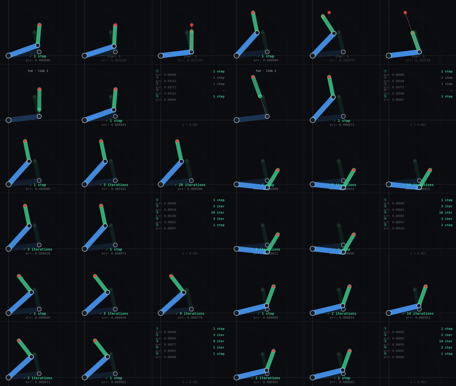
Here is a recap of the 5 approaches to inverse kinematics:
Some require only 1 iteration but need more upfront work (analytical, learning-based).
Others are straightforward to apply but require convergence over multiple iterations.
Bonus:
- Can you find a target for which the solved configuration is different for some approaches?
- Can you find a target that needs more iterations for CCD vs FABRIK and vice-versa?
Write your findings in the comment section below 👇